358168
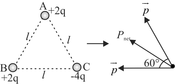
Electric charges \(2q,2q, - 4q\) are placed at the corners of an equilateral \(\Delta \,ABC\) of side \(l\). The magnitude of electric dipole moment of the system is
1 \(\,ql\)
2 \(\sqrt 3 \,ql\)
3 \(2\sqrt 3 ql\)
4 \(\sqrt 2 \,ql\)
Explanation:
The dipole moments of the combination is shown in the following figure The charge \( - 4q\) can be considered as a combination of two charges each of charge \( - 2q\). So \( + 2q\) forms dipole with \( - 2q\) . So we have two dipoles. Net dipole moment, i.e., \({p_{net}} = \sqrt {{p^2} + {p^2} + 2pp\,\,\cos \,\,60^\circ } = \sqrt 3 p\) \( = \sqrt 3 \left( {2ql} \right) = 2\sqrt 3 ql\left( {p = ql} \right)\)
PHXII01:ELECTRIC CHARGES AND FIELDS
358169
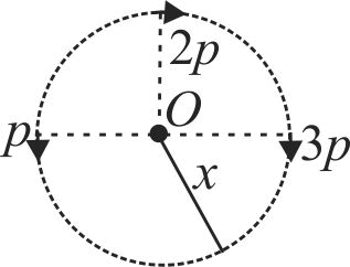
Three small dipoles are arranged as shown below. What will be the net electric field at point \(O\left( {k = \frac{1}{{4\pi {\varepsilon _0}}}} \right)\)
1 \(\sqrt 5 \frac{{kp}}{{{x^3}}}\)
2 \(2\sqrt 5 \frac{{kp}}{{{x^3}}}\)
3 \(\frac{{5kp}}{{{x^3}}}\)
4 \(0\)
Explanation:
The fields produced by the three dipoles are \({{\vec E}_1} = \frac{{ - kp}}{{{x^3}}}\hat j,{{\vec E}_2} = \frac{{ - k\left( {2p} \right)}}{{{x^3}}}\hat i,{{\vec E}_3} = \frac{{ - k\left( {3p} \right)}}{{{x^3}}}\hat j\) \({{\vec E}_{net}} = {{\vec E}_1} + {{\vec E}_2} + {{\vec E}_3} = \frac{{ - 2kp}}{{{x^3}}}\hat i - \frac{{4kp}}{{{x^3}}}\hat j\) \({{\vec E}_{net}} = 2\sqrt 5 \frac{{kp}}{{{x^3}}}\)
PHXII01:ELECTRIC CHARGES AND FIELDS
358170
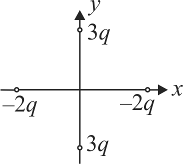
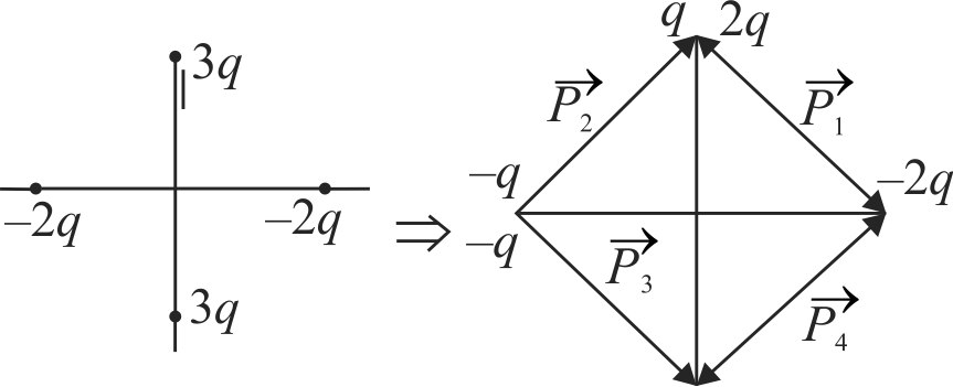
4 charges are placed each at a distance ' \(a\) ' from origin. The dipole moment of configuration is :
1 \(2 q a \hat{j}\)
2 \(3 q a \hat{j}\)
3 \(2 a q[\hat{i}+\hat{j}]\)
4 None of these
Explanation:
\(P_{3}=P_{3}=\sqrt{2} q a ; P_{1}=2 \sqrt{2} q a\) Here \(p_{x}=0\) and \(p_{y}=2 q a\) \(\Rightarrow \vec{p}_{n e t}=2 q a \hat{j}\)
PHXII01:ELECTRIC CHARGES AND FIELDS
358171
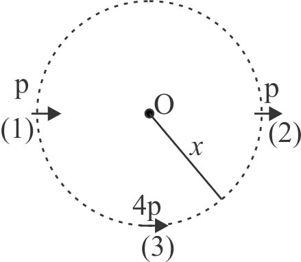
Three small dipoles are arranged as shown below. What will be the net electric field at \(O\left( {k = \frac{1}{{4\pi {\varepsilon _0}}}} \right)\)
1 \(\frac{{8kp}}{{{x^3}}}\)
2 \(\frac{{kp}}{{{x^3}}}\)
3 \(\frac{{\sqrt 2 kp}}{{{x^3}}}\)
4 Zero
Explanation:
Point \(O\) lies at axial positions of dipole 1 and 2 and equatorial position of dipole 3. Hence field at \(O\) is \({E_1} = \frac{{k2p}}{{{x^3}}}\) (towards right) due to dipole 1 \({E_2} = \frac{{k2p}}{{{x^3}}}\) (towards right) due to dipole 2 \({E_3} = \frac{{k\left( {4p} \right)}}{{{x^3}}}\) (towards left) due to dipole 3 The net field at \(P\) is zero.
358168
Electric charges \(2q,2q, - 4q\) are placed at the corners of an equilateral \(\Delta \,ABC\) of side \(l\). The magnitude of electric dipole moment of the system is
1 \(\,ql\)
2 \(\sqrt 3 \,ql\)
3 \(2\sqrt 3 ql\)
4 \(\sqrt 2 \,ql\)
Explanation:
The dipole moments of the combination is shown in the following figure The charge \( - 4q\) can be considered as a combination of two charges each of charge \( - 2q\). So \( + 2q\) forms dipole with \( - 2q\) . So we have two dipoles. Net dipole moment, i.e., \({p_{net}} = \sqrt {{p^2} + {p^2} + 2pp\,\,\cos \,\,60^\circ } = \sqrt 3 p\) \( = \sqrt 3 \left( {2ql} \right) = 2\sqrt 3 ql\left( {p = ql} \right)\)
PHXII01:ELECTRIC CHARGES AND FIELDS
358169
Three small dipoles are arranged as shown below. What will be the net electric field at point \(O\left( {k = \frac{1}{{4\pi {\varepsilon _0}}}} \right)\)
1 \(\sqrt 5 \frac{{kp}}{{{x^3}}}\)
2 \(2\sqrt 5 \frac{{kp}}{{{x^3}}}\)
3 \(\frac{{5kp}}{{{x^3}}}\)
4 \(0\)
Explanation:
The fields produced by the three dipoles are \({{\vec E}_1} = \frac{{ - kp}}{{{x^3}}}\hat j,{{\vec E}_2} = \frac{{ - k\left( {2p} \right)}}{{{x^3}}}\hat i,{{\vec E}_3} = \frac{{ - k\left( {3p} \right)}}{{{x^3}}}\hat j\) \({{\vec E}_{net}} = {{\vec E}_1} + {{\vec E}_2} + {{\vec E}_3} = \frac{{ - 2kp}}{{{x^3}}}\hat i - \frac{{4kp}}{{{x^3}}}\hat j\) \({{\vec E}_{net}} = 2\sqrt 5 \frac{{kp}}{{{x^3}}}\)
PHXII01:ELECTRIC CHARGES AND FIELDS
358170
4 charges are placed each at a distance ' \(a\) ' from origin. The dipole moment of configuration is :
1 \(2 q a \hat{j}\)
2 \(3 q a \hat{j}\)
3 \(2 a q[\hat{i}+\hat{j}]\)
4 None of these
Explanation:
\(P_{3}=P_{3}=\sqrt{2} q a ; P_{1}=2 \sqrt{2} q a\) Here \(p_{x}=0\) and \(p_{y}=2 q a\) \(\Rightarrow \vec{p}_{n e t}=2 q a \hat{j}\)
PHXII01:ELECTRIC CHARGES AND FIELDS
358171
Three small dipoles are arranged as shown below. What will be the net electric field at \(O\left( {k = \frac{1}{{4\pi {\varepsilon _0}}}} \right)\)
1 \(\frac{{8kp}}{{{x^3}}}\)
2 \(\frac{{kp}}{{{x^3}}}\)
3 \(\frac{{\sqrt 2 kp}}{{{x^3}}}\)
4 Zero
Explanation:
Point \(O\) lies at axial positions of dipole 1 and 2 and equatorial position of dipole 3. Hence field at \(O\) is \({E_1} = \frac{{k2p}}{{{x^3}}}\) (towards right) due to dipole 1 \({E_2} = \frac{{k2p}}{{{x^3}}}\) (towards right) due to dipole 2 \({E_3} = \frac{{k\left( {4p} \right)}}{{{x^3}}}\) (towards left) due to dipole 3 The net field at \(P\) is zero.